Notes on domain-specific ChatGPT

Mar 25 2023

Last updated on July 14 2025

What are Vector Embeddings?

Vector embeddings are central to many NLP, recommendation, and search algorithms. We create vector embeddings, which are just lists of numbers, to perform various operations with them. A whole paragraph of text or any other object can be reduced to a vector.

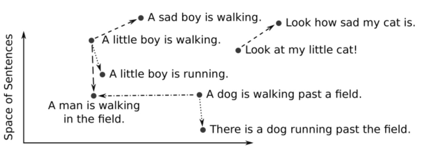
There is something special about vectors that makes them so useful. This representation makes it possible to translate semantic similarity as perceived by humans to proximity in a vector space. In other words, when we represent real-world objects and concepts such as images, audio recordings, news articles, and user profiles as vector embeddings, the semantic similarity of these objects and concepts can be quantified by how close they are to each other as points in vector spaces.

We train models to translate objects to vectors. A deep neural network is a common tool for training such models. The resulting embeddings are usually high dimensional (up to two thousand dimensions) and dense (all values are non-zero). For text data, models such as Word2Vec, GloVe (Global Vectors for Word Representation), and BERT transform words, sentences, or paragraphs into vector embeddings. Images can be embedded using models such as convolutional neural networks (CNNs).

Tokens and Embeddings

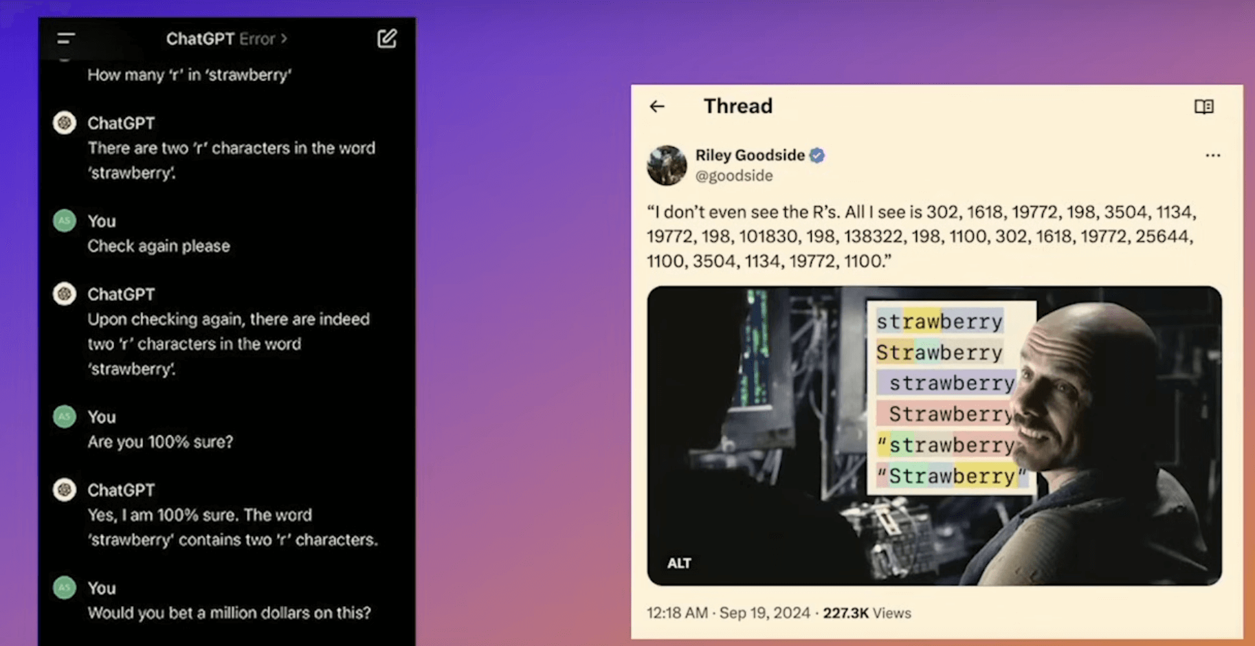
Tokens are the basic units of data processed by LLMs. In the context of text, a token can be a word, part of a word (subword), or even a character — depending on the tokenization process.

In the context of GPT, each piece of text is represented by the ID of the corresponding token in the final vocabulary. If a word is not in the vocabulary, it’s broken down into smaller tokens that are in the vocabulary. The key point is that the assignment of token IDs is not arbitrary but based on the frequency of occurrence and combination patterns in the language data the model was trained on.

# Online playground for OpenAPI tokenizers: https://tiktokenizer.vercel.app
# Tokenizer - OpenAI API: https://platform.openai.com/tokenizer

"Apple is a fruit"

-> ['Apple', ' is', ' a', ' fruit']
-> [32352, 382, 261, 15310]

// npm install js-tiktoken
// This is a pure JS port of the original tiktoken library.

import { Tiktoken } from "js-tiktoken/lite";
import o200k_base from "js-tiktoken/ranks/o200k_base";

const enc = new Tiktoken(o200k_base);
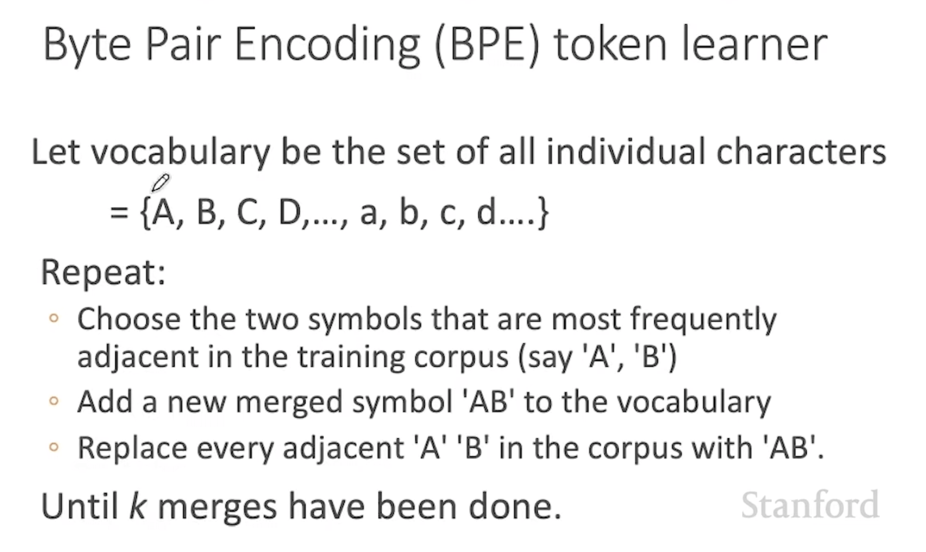
assert(enc.decode(enc.encode("hello world")) === "hello world");

Language models don’t see text like you and I, instead they see a sequence of tokens. Byte pair encoding (BPE) is a way of converting text into tokens used in GPT.

It’s reversible and lossless, so you can convert tokens back into the original text.

It compresses the text: the token sequence is shorter than the bytes corresponding to the original text. On average, in practice, each token corresponds to about 4 bytes.

It attempts to let the model see common subwords. For instance, “ing” is a common subword in English, so BPE encodings will often split “encoding” into tokens like “encod” and “ing” (instead of e.g. “enc” and “oding”). Because the model will then see the “ing” token again and again in different contexts, it helps models generalise and better understand grammar.

It ensures that the most common words are represented as a single token while the rare words are broken down into two or more subword tokens. (Looking for the most frequent pairing, merge them, and perform the same iteration again and again until we reach our token limit or iteration limit.)

Embeddings are advanced vector representations of tokens. They try to capture the most nuance, connections, and semantic meanings between tokens. Each embedding is generally a series of real numbers on a vector space computed by a neural network. They are the “real inputs” of LLMs.

If you load a model from libraries, the embedding table is included automatically as part of the model’s weights. The model looks up each token ID in the embedding table (Token Embedding Matrix) to get token embeddings. These are token-level embeddings. To get an embedding for the whole sentence, you need to combine these token embeddings into one vector that represents the full sentence, which yields a sentence-level embedding.

Token embeddings alone do not capture word order, models add positional information (Position Embedding Matrix) to embeddings. In general, we use the postion in the prompt to define a samll offset to the token’s embeddings to slightly move it in the embedding space.

from langchain_openai.embeddings import OpenAIEmbeddings

embeddings = OpenAIEmbeddings()
embedded_query = embeddings.embed_query("Who is Mary's sister?")

print(f"Embedding length: {len(embedded_query)}") # Embedding length: 1536
print(embedded_query) # [-0.0013594045786472937, -0.03437049808954925, ...]

In data analysis, cosine similarity is a measure of similarity between two non-zero vectors defined in an inner product space. Cosine similarity is the cosine of the angle between the vectors; that is, it is the dot product of the vectors divided by the product of their lengths.

Self Attention Mechanism

Tokenaizer -> Embedding (capture semantic meaning) -> Attention (capture contextual meaning)

Embeddings alone don’t distinguish between words with multiple meanings. Embedding table assigns a signle vector regardless of the context. This is where self-attention comes in. Self attention mechanism transforms semantic representations into context-aware representations making words are understood in the context of the sentence.

Each token’s embedding is multiplied by three learned weight matrices to produce three vectors:

Query (Q): “What am I looking for from other tokens?”
Key (K): “This is what I offer to tokens looking at me.”
Value (V): “This is the information I pass along if there’s a match.”

Example

Sentence: “The cat that I saw yesterday was sleeping.”

When the model computes the new representation for “was”, it follows these steps:

Query construction: “was” is projected through the learned matrix to produce its Query vector. Semantically, this vector encodes something like “I am a verb; I need to find my subject.”
Key comparison: Q is compared, via dot product, against the Key vector of every token in its attention window: “The”, “cat”, “that”, “I”, “saw”, “yesterday”. Each comparison produces a scalar score — a measure of how well that token’s Key aligns with what “was” is looking for.
- The score for “cat” is large, because the model has learned that Key vectors for nouns in subject position align well with the Query pattern of a following verb.
- The score for “yesterday” is small, because temporal adverbs don’t produce Keys that match a “find my subject” Query.
Scaling and softmax: each score is divided by a constant based on the dimensionality of the Key vectors, to keep the numbers in a stable range. The scaled scores are then passed through softmax, which converts them into a probability distribution — a set of weights that are all non-negative and sum to 1. Suppose this yields approximately:
- cat → 0.70
- saw → 0.10
- I → 0.08
- yesterday → 0.04
- The → 0.04
- that → 0.04
Weighted sum of Values: each token also has a Value vector. To build the new representation for “was”, each token’s Value vector is scaled by its corresponding weight. Then, all six scaled Value vectors are added together component by component. For intuition, imagine each Value vector has just 3 dimensions:
- V_cat = [2, 0, 4], weight 0.70 → scaled = [1.4, 0, 2.8]
- V_saw = [0, 1, 0], weight 0.10 → scaled = [0, 0.1, 0]
- V_I = [1, 1, 1], weight 0.08 → scaled = [0.08, 0.08, 0.08]
- (similarly small contributions from “yesterday”, “The”, “that”)
Adding these scaled vectors position-by-position gives approximately:

new_was ≈ [1.5, 0.2, 2.9]

Because the weight for “cat” dominates (0.70), new_was ends up very close to V_cat = [2, 0, 4], with small nudges from the other tokens’ Values blended in.

new_was — the new representation of “was” — now encodes “this verb’s subject is the cat,” even though “cat” is six tokens away in the sequence. This is the mechanism by which self-attention resolves long-range dependencies: not through position or distance, but through learned similarity between Query and Key vectors.

This is just one attention layer. Transformers stack many of these layers. So new_was from layer 1 becomes the input embedding for layer 2, gets transformed into Q/K/V again, attends again, and produces an even more refined representation. By the final layer, “was” might encode something very rich — subject, tense, surrounding clause structure, etc.

An attention head is one independent attention pass with its own learned projections. Each head runs its attention pass independently. Then the outputs of all the heads get concatenated and passed through a final linear layer that mixes them back into one full-size vector.

When generating token N+1: The model only computes Q, K, V for the new token. It reuses the already-stored K and V vectors for tokens 1 through N from the cache. This is called the KV cache. It saves the model from recomputing the whole prompt every time it adds a token. (Also see Prompt caching)

Storing embeddings in Postgres with pgvector

How can I retrieve K nearest embedding vectors quickly? For searching over many vectors quickly, we recommend using a vector database.

pgvector is an open-source vector similarity search for Postgres. Once we have generated embeddings on multiple texts, it is trivial to calculate how similar they are using vector math operations like cosine distance. A perfect use case for this is search. Your process might look something like this:

Pre-process your knowledge base and generate embeddings for each page.
Store your embeddings.
Build a search page that prompts your user for input.
Take user’s input, generate a one-time embedding, then perform a similarity search against your pre-processed embeddings.
Return the most similar pages to the user.

pgvector introduces a new data type called vector. We create a column named embedding with the vector data type. The size of the vector defines how many dimensions the vector holds. OpenAI’s text-embedding-ada-002 model outputs 1536 dimensions, so we will use that for our vector size. We also create a text column named content to store the original document text that produced this embedding. Depending on your use case, you might just store a reference (URL or foreign key) to a document here instead.

create table documents (
  id bigserial primary key,
  content text,
  embedding vector (1536)
);

ChatGPT doesn’t just return existing documents. It’s able to assimilate a variety of information into a single, cohesive answer. To do this, we need to provide GPT with some relevant documents, and a prompt that it can use to formulate this answer.

One of the biggest challenges of OpenAI’s text-davinci-003 completion model is the 4000 token limit. This makes it challenging if you wanted to prompt GPT-3 to answer questions about your own custom knowledge base that would never fit in a single prompt. Embeddings can help solve this by splitting your prompts into a two-phased process:

Query your embedding database for the most relevant documents related to the question.
Inject these documents as context for GPT-3 to reference in its answer.

// https://supabase.com/blog/openai-embeddings-postgres-vector

// Generate a one-time embedding for the query itself
const embeddingResponse = await openai.createEmbedding({
  model: "text-embedding-ada-002",
  input,
});

const [{ embedding }] = embeddingResponse.data.data;

// Fetching whole documents for this simple example.
// `match_documents` is a function to perform similarity search over embeddings
const { data: documents } = await supabaseClient.rpc("match_documents", {
  query_embedding: embedding,
  match_threshold: 0.78, // Choose an appropriate threshold for your data
  match_count: 10, // Choose the number of matches
});

const tokenizer = new GPT3Tokenizer({ type: "gpt3" });
let tokenCount = 0;
let contextText = "";

// Concat matched documents
for (let i = 0; i < documents.length; i++) {
  const document = documents[i];
  const content = document.content;
  const encoded = tokenizer.encode(content);
  tokenCount += encoded.text.length;

  // Limit context to max 1500 tokens (configurable)
  if (tokenCount > 1500) {
    break;
  }

  contextText += `${content.trim()}\n---\n`;
}

const prompt = stripIndent`${oneLine`
  You are a very enthusiastic Supabase representative who loves
  to help people! Given the following sections from the Supabase
  documentation, answer the question using only that information,
  outputted in markdown format. If you are unsure and the answer
  is not explicitly written in the documentation, say
  "Sorry, I don't know how to help with that."`}

  Context sections:
  ${contextText}

  Question: """
  ${query}
  """

  Answer as markdown (including related code snippets if available):
`;

const completionResponse = await openai.createCompletion({
  model: "text-davinci-003",
  prompt,
  max_tokens: 512, // Choose the max allowed tokens in completion
  temperature: 0, // Set to 0 for deterministic results
});

Domain-specific ChatGTP Starter App

This starter app uses embeddings to generate a vector representation of a document, and then uses vector search to find the most similar documents to the query. The results of the vector search are then used to construct a prompt for GPT-3, which is then used to generate a response. The response is then streamed to the user.

Creating and storing the embeddings: See pages/embeddings.tsx and pages/api/generate-embeddings.ts

Web pages are scraped, stripped to plain text and split into 1000-character documents.
OpenAI’s embedding API is used to generate embeddings for each document using the text-embedding-ada-002 model.
The embeddings are then stored in a Supabase postgres table using pgvector.

Responding to queries: See pages/api/docs.ts and utils/OpenAIStream.ts

A single embedding is generated from the user prompt.
That embedding is used to perform a similarity search against the vector database.
The results of the similarity search are used to construct a prompt for GPT-3.
The GTP-3 response is then streamed to the user.

// generate and store embeddings from a list of input URLs
const { method, body } = req;
const { urls } = body;
const documents = await getDocuments(urls);

for (const { url, body } of documents) {
  const input = body.replace(/\n/g, " ");

  const embeddingResponse = await openAi.createEmbedding({
    model: "text-embedding-ada-002",
    input
  });

  const [{ embedding }] = embeddingResponse.data.data;

  await supabaseClient.from("documents").insert({
    content: input,
    embedding,
    url
  });
}

const docSize: number = 1000;  // embedding doc sizes

async function getDocuments(urls: string[]) {
  const documents = [];
  for (const url of urls) {
    const response = await fetch(url);
    const html = await response.text();
    const $ = cheerio.load(html);
    const articleText = $("body").text();

    let start = 0;
    while (start < articleText.length) {
      const end = start + docSize;
      const chunk = articleText.slice(start, end);
      documents.push({ url, body: chunk });
      start = end;
    }
  }
  return documents;
}

GPT and LangChain Chatbot for PDF docs

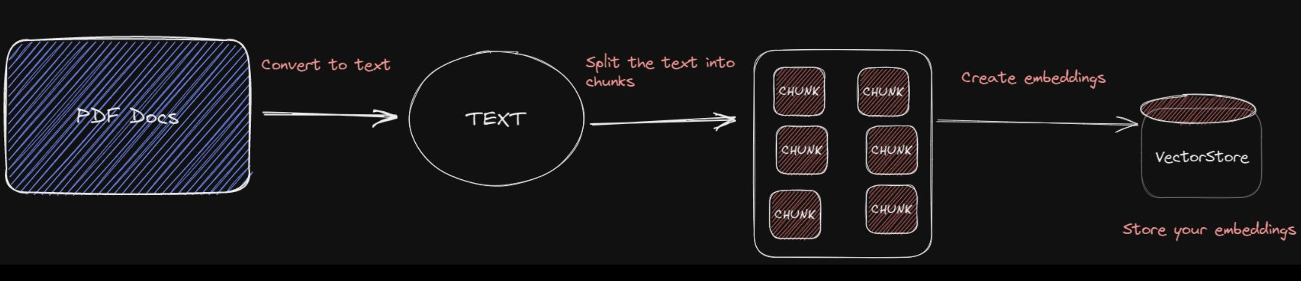
gpt4-pdf-chatbot-langchain uses LangChain and Pinecone to build a chatbot for large PDF docs. Convert your PDF to embeddings:

// https://github.com/mayooear/gpt4-pdf-chatbot-langchain/blob/main/scripts/ingest-data.ts

/* load raw docs from the pdf file in the directory */
// https://js.langchain.com/docs/modules/indexes/document_loaders/examples/file_loaders/pdf
const loader = new PDFLoader(filePath);
const rawDocs = await loader.load();

/* split text into chunks */
// https://js.langchain.com/docs/modules/indexes/text_splitters/examples/recursive_character
const textSplitter = new RecursiveCharacterTextSplitter({
  chunkSize: 1000,
  chunkOverlap: 200,
});
const docs = await textSplitter.splitDocuments(rawDocs);

/* create and store the embeddings in the vectorStore */
// https://js.langchain.com/docs/modules/models/embeddings/integrations
const embeddings = new OpenAIEmbeddings();

// https://github.com/hwchase17/langchainjs/pull/112
const pinecone = new PineconeClient();
await pinecone.init({
  environment: process.env.PINECONE_ENVIRONMENT,
  apiKey: process.env.PINECONE_API_KEY,
});
// An index is the highest-level organizational unit of vector data in Pinecone.
// It accepts and stores vectors, serves queries over the vectors it contains,
// and does other vector operations over its contents.
const index = pinecone.Index(PINECONE_INDEX_NAME); // change to your own index name

/* embed the PDF documents */
const chunkSize = 50;
for (let i = 0; i < docs.length; i += chunkSize) {
  const chunk = docs.slice(i, i + chunkSize);
  await PineconeStore.fromDocuments(index, chunk, embeddings);
}

Vector Database

Vector Databases Explained: https://vercel.com/guides/vector-databases
What is a Vector Database: https://www.pinecone.io/learn/vector-database

Several algorithms can facilitate the creation of a vector index. Their goal is to enable fast querying by creating a data structure that can be traversed quickly. They will commonly transform the representation of the original vector into a compressed form to optimize the query process.

HNSW (Hierarchical Navigable Small World) creates a hierarchical, tree-like structure where each node of the tree represents a set of vectors. The edges between the nodes represent the similarity between the vectors. The algorithm starts by creating a set of nodes, each with a small number of vectors. The algorithm then examines the vectors of each node and draws an edge between that node and the nodes that have the most similar vectors to the one it has. When we query an HNSW index, it uses this graph to navigate through the tree, visiting the nodes that are most likely to contain the closest vectors to the query vector.

Techniques beyond basic RAG

There is more to RAG than putting documents into a vector DB and adding an LLM on top. That can work, but it won’t always. The retrieval may return relevant information below our top_k cutoff. The metric we would measure here is recall, which measures how many relevant documents are retrieved out of the total number of relevant documents in the dataset. LLM recall degrades as we put more tokens in the context window.

A reranking model — also known as a cross-encoder — is a type of model that, given a query and document pair, will output a similarity score. We use this score to reorder the documents by relevance to our query. Search engineers have used rerankers in two-stage retrieval systems for a long time. In these two-stage systems, a first-stage model (an embedding model / bi-encoder) retrieves a set of relevant documents from a larger dataset. Then, a second-stage model (the reranker) is used to rerank those documents retrieved by the first-stage model. Note that rerankers are slow, and retrievers are fast.

bi-encoders must compress all of the possible meanings of a document into a single vector — meaning we lose information. Additionally, bi-encoders have no context on the query because we don’t know the query until we receive it (we create embeddings before user query time).
A cross-encoder is a type of neural network architecture used in NLP tasks, particularly in the context of sentence or text pair classification. Its purpose is to evaluate and provide a single score for a pair of input sentences, indicating the relationship or similarity between them. Cross-encoders are more accurate than bi-encoders but they don’t scale well, so using them to re-order a shortened list returned by semantic search is the ideal use case.

# https://www.sbert.net/docs/cross_encoder/pretrained_models.html
from sentence_transformers import CrossEncoder
import torch

model = CrossEncoder("cross-encoder/ms-marco-MiniLM-L-6-v2", default_activation_function=torch.nn.Sigmoid())
scores = model.predict([
    ("How many people live in Berlin?", "Berlin had a population of 3,520,031 registered inhabitants in an area of 891.82 square kilometers."),
    ("How many people live in Berlin?", "Berlin is well known for its museums."),
])
# => array([0.9998173 , 0.01312432], dtype=float32)

Rerank APIs

JinaAI Reranker (1 million free tokens): https://jina.ai/reranker
Cohere offers an API for reranking documents: https://cohere.com/blog/rerank

Jina AI Search Foundation Models:

Embedding Models: jina-embeddings-v3, jina-embeddings-v4(multimodal and multilingual)

Reranker Models: jina-reranker-v2-base-multilingual

Small Language Models (SLMs): ReaderLM-v2

Query Transformation

RAG systems often face challenges in retrieving the most relevant information, especially when dealing with complex or ambiguous queries. These query transformation techniques address this issue by reformulating queries to better match relevant documents or to retrieve more comprehensive information.

Query Rewriting: Reformulates queries to be more specific and detailed.
Step-back Prompting: Generates broader queries for better context retrieval.
Sub-query Decomposition: Breaks down complex queries into simpler sub-queries.

DeepSearch and DeepResearch

https://jina.ai/news/a-practical-guide-to-implementing-deepsearch-deepresearch/

DeepSearch runs through an iterative loop of searching, reading, and reasoning until it finds the optimal answer.
DeepResearch builds upon DeepSearch by adding a structured framework for generating long research reports.

RAG is about answering questions that fall outside of the knowledge baked into a model. The DeepSearch pattern offers a tools-based alternative to classic RAG: we give the model extra tools for running multiple searches and run it for several steps in a loop to try to find an answer.

Kexi's blog

blog/notes/digital garden